R语言空间数据综合制图

空间数据的简单可视化通常不能直接作为论文配图,一张标准的地图还需要考虑投影、比例尺、指北针等制图要素。本文展示了一张标准地图的生产过程。可视化内容请参考前一篇post——R语言空间数据可视化 | Xiaoran Wu。
首先加载将使用到的packages:
sf:矢量数据处理
ggplot2:绘图地图
ggspatial:绘制比例尺、指北针
cowplot:拼接主图与子图
library(sf)
library(ggplot2)
library(ggspatial)
library(cowplot)
再加载将使用到的数据:
Boundary_China <- st_read('Boundary_China.shp')
Boundary_Heihe <- st_read('Boundary_Heihe.shp')
Jiuduanxian <- st_read('Jiuduanxian.shp')
Nanhai <- st_read('Nanhai.shp')

Boundary_Heihe$name <- "Heihe river basin"
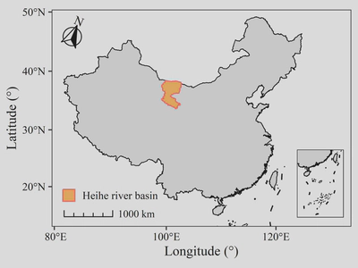
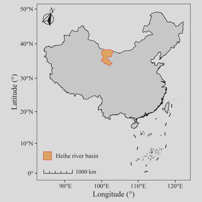
使用以下代码,可生成一幅仅被可视化的地图。
ggplot()+
  geom_sf(data = Boundary_China,
          linewidth = 0.3,
          color = "black")+
  geom_sf(data = Boundary_Heihe,
          aes(color = name),
          fill = "#ffb75e",
          linewidth = 0.5) +
  geom_sf(data = Jiuduanxian)+
  geom_sf(data = Nanhai,
          linewidth = 0.3,
          color = "black")+
  coord_sf(crs = st_crs(4236)) +
  scale_color_manual(values = "#ff645e") +
  labs(x = "Longitude (°)",
       y = "Latitude (°)",
       color = NULL) +
  theme_bw() +
  theme(text = element_text(family = "serif"),
        axis.text = element_text(color = "black"),
        panel.grid = element_blank(),
        legend.position = c(0.17,0.07),
        legend.key.size = unit(13, "pt"))
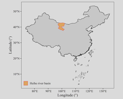
一、投影
改变地图投影的函数是coord_sf(),函数中的crs参数可以使用PROJ4字符串或ESPG码。如原图中使用了ESPG码(4236)来使用WGS84投影。
Albers是我国常用的地图投影之一。中国所使用的Albers的参数是双标准纬线(25°N与47°N)中央经线为105°E,椭球体为Krassovsky。用PROJ4表示为“+proj=aea +ellps=krass +lon_0=105 +lat_1=25 +lat_2=47”。
使用以下代码替换原图的投影:
coord_sf(crs = "+proj=aea +ellps=krass +lon_0=105 +lat_1=25 +lat_2=47")
生成的新图效果如下:
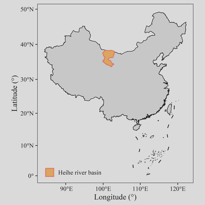
二、指北针
annotation_north_arrow()函数可以为图片添加指北针。其中主要设置的属性如下:
location:相对位置,上左为“tl”,下右为“br”,以此类推;
pad_x/pad_y:设置横向/纵向的偏移,以unit()函数构建;
height/width:指北针的高度与宽度,以unit()函数构建;
which_north:指北针的北所指的方向,“grid”为图面的北,“true”为坐标系北;
style:指北针样式,共四个样式,可通过样式同名函数构建来自定义样式。
在前一幅图的代码中添加以下代码增加指北针:
annotation_north_arrow(location = "tl",
                       pad_x = unit(5, "pt"),
                       pad_y = unit(7, "pt"),
                       height = unit(25, "pt"),
                       width = unit(25, "pt"),
                       which_north = "true",
                       style = north_arrow_fancy_orienteering(text_family = "serif"))
三、比例尺
annotation_scale()函数用于创建比例尺。主要的属性设置如下:
location:相对位置,上左为“tl”,下右为“br”,以此类推;
pad_x/pad_y:设置横向/纵向的偏移,以unit()函数构建;
height:比例尺的高度,以unit()函数构建;
width_hint:比例尺的宽度,为比例尺占图面宽度的比例;
style:比例尺样式,有“bar”与“ticks”;
unit_category:设置比例尺的单位,“metric”公制,“imperial”英制;
text_*:与字体相关的设置
在前一幅图的代码中添加以下代码增加比例尺:
annotation_scale(location = "bl",
                 pad_x = unit(10, "pt"),
                 pad_y = unit(10, "pt"),
                 height = unit(5, "pt"),
                 width_hint = 0.2,
                 style = "ticks",
                 unit_category = "metric",
                 text_family = "serif",
                 line_width = 1)
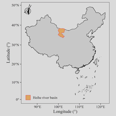
四、子图
当绘制中国地图时常常需要补充一个南海区域的小图,而美国地图则需要补充阿拉斯加半岛的小图,有时候则是补充一个鹰眼视图,原理是相同的。
先绘制好两个图,都需要在coord_sf()函数中使用xlim和ylim属性设置图面范围;再使用cowplot包中的draw_plot()函数逐个绘制,x与y属性设置子图左下角在主图中的位置,height和width属性分别设置子图的高度与宽度。
子图绘制的完整代码如下:
main_polt <- ggplot()+
  geom_sf(data = Boundary_China,
          linewidth = 0.3,
          color = "black") +
  geom_sf(data = Boundary_Heihe,
          aes(color = name),
          fill = "#ffb75e",
          linewidth = 0.5) +
  geom_sf(data = Jiuduanxian) +
  geom_sf(data = Nanhai,
          linewidth = 0.3,
          color = "black") +
  annotation_north_arrow(location = "tl",
                         pad_x = unit(5, "pt"),
                         pad_y = unit(7, "pt"),
                         height = unit(25, "pt"),
                         width = unit(25, "pt"),
                         which_north = "true",
                         style = north_arrow_fancy_orienteering(text_family = "serif")) +
  annotation_scale(location = "bl",
                   pad_x = unit(10, "pt"),
                   pad_y = unit(8, "pt"),
                   height = unit(5, "pt"),
                   width_hint = 0.2,
                   style = "ticks",
                   unit_category = "metric",
                   text_family = "serif",
                   line_width = 1,
  ) +
  coord_sf(crs = "+proj=aea +ellps=krass +lon_0=105 +lat_1=25 +lat_2=47",
           ylim = c(1851151, 5863805),
           xlim = c(-2601944, 2924108))+
  scale_color_manual(values = "#ff645e") +
  labs(x = "Longitude (°)",
       y = "Latitude (°)",
       color = NULL) +
  theme_bw() +
  theme(text = element_text(family = "serif"),
        axis.text = element_text(color = "black"),
        panel.grid = element_blank(),
        legend.position = c(0.197,0.16),
        legend.key.size = unit(11, "pt"),
        legend.background = element_blank())

sub_plot <- ggplot()+
  geom_sf(data = Boundary_China,
          linewidth = 0.3,
          color = "black") +
  geom_sf(data = Jiuduanxian) +
  geom_sf(data = Nanhai,
          linewidth = 0.3,
          color = "black") +
  coord_sf(crs = "+proj=aea +ellps=krass +lon_0=105 +lat_1=25 +lat_2=47",
           ylim = c(370910,2809416),
           xlim = c(200000,1870662))+
  theme_void() +
  theme(panel.border = element_rect(fill = "transparent"))

ggdraw() +
  draw_plot(main_polt) +
  draw_plot(sub_plot, x = 0.83, y = 0.16, width = 0.13, height = 0.39)
子图的绘制效果,也即本文考虑全部制图要素后绘制的标准地图如下: